Gods estimator of mean rarity
Gods_estimator.RmdHill diversities (also called “Hill numbers”) have become standard
for measuring diversity in ecology (cite the Ellison 2010 special
issue). While many interpretations of Hill numbers have been discussed,
including their relationship to species richness, Shannon’s entropy, and
Simpson’s concentration, The package MeanRarity is designed
to illustrate an alternative interpretation of Hill numbers as means of
species rarity (the reciprocal of relative abundance) in a community. In
this interpretation, the control parameter \(\ell\) moves the index from arithmetic to
geometric to harmonic means. Thus, Hill diversities differ in the scale
on which species rarity is considered, but always weights species the
same way (by their abundance) regardless of the scale being used. This
interpretation is distinct from the common idea that the Hill parameter
controls how rare vs. common species are “weighted.”
In this vignette, we show that the mean rarity perspective suggests a novel approach to estimating true diversity from a sample, using the fact that the sample mean is an unbiased estimate of the population mean. Although how to estimate a species’ rarity from sample data remains unsolved, we test the promise of this idea using what we call God’s estimator: All-knowing, God can plug in the true population parameters for each species. Nevertheless, maybe for fun, God chooses to compute the sample mean, weighting species’ true rarities by their sampled frequency.
Let’s see how God’s estimator works!
First, we simulate some SADs with known diversity using the function
fit_SAD()
# simulate SADs for analysis
SADs_list<-map(c("lnorm", "gamma"), function(distr){
  map(c(100, 200), function(rich){
    map(c(.1,.15,.25,.5,0.75,.85), function(simp_Prop){ #simp_Prop is evenness
      fit_SAD(rich = rich, simpson = simp_Prop*(rich-1)+1, distr = distr)
    })
  })
})
#> Warning in fit_SAD(rich = rich, simpson = simp_Prop * (rich - 1) + 1, distr = distr): Rarest species has relative abundance  1.73323975748106e-23 .
#> Consider implied community size.
#> Warning in fit_SAD(rich = rich, simpson = simp_Prop * (rich - 1) + 1, distr = distr): Rarest species has relative abundance  1.20738866916925e-15 .
#> Consider implied community size.
#> Warning in fit_SAD(rich = rich, simpson = simp_Prop * (rich - 1) + 1, distr = distr): Rarest species has relative abundance  1.7925645196612e-09 .
#> Consider implied community size.
#> Warning in fit_SAD(rich = rich, simpson = simp_Prop * (rich - 1) + 1, distr = distr): Rarest species has relative abundance  1.83050169167485e-26 .
#> Consider implied community size.
#> Warning in fit_SAD(rich = rich, simpson = simp_Prop * (rich - 1) + 1, distr = distr): Rarest species has relative abundance  1.36083992426459e-17 .
#> Consider implied community size.
#> Warning in fit_SAD(rich = rich, simpson = simp_Prop * (rich - 1) + 1, distr = distr): Rarest species has relative abundance  1.21155246166886e-10 .
#> Consider implied community size.
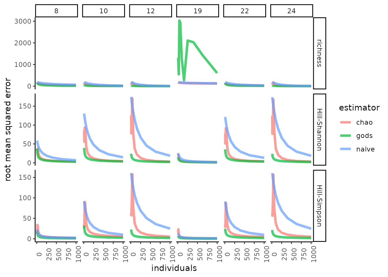
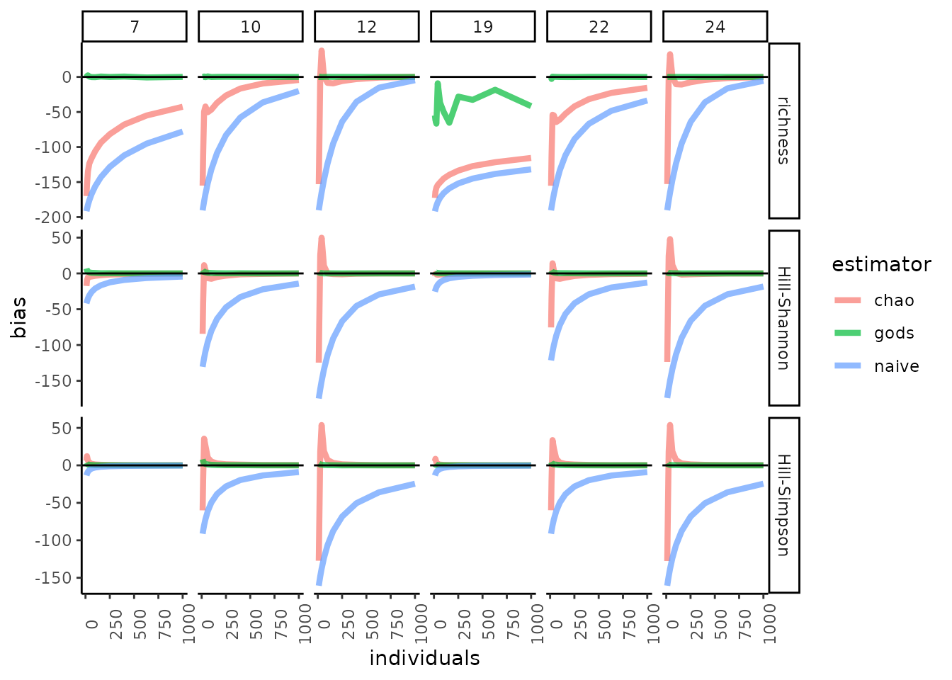
Now, let’s test estimator performance.We’ll compare what we’ve called “God’s estimator” to the naïve estimator (the mean of the observed rarities) and to a non-parametric, asymptotic diversity estimator (CITE Chao and Jost 2015). To assess performance, let’s look at the root mean squared error, and also bias.
We won’t run the first part as it could take a while.
nreps <- 9999

ss_to_test <- floor(10^seq(1,3, 0.2))

flatsads <- flatten(flatten(SADs_list))

nc <- parallel::detectCores() - 1
future::plan(strategy = "multiprocess", workers = nc)
# options <- furrr::furrr_options(seed = TRUE)
tic()
compare_ests <- map_dfr(1:24, function(SAD){
  map_dfr(-1:1, function(ell){
   truth = as.numeric(flatsads[[SAD]][[2]][2-ell])
   truep = flatsads[[SAD]][[3]]
   dinfo = data.frame(t(flatsads[[SAD]][[1]]))
  future_map_dfr(.x=1:nreps, .f=function(nrep){
      map_dfr(ss_to_test, function(ss){
        subsam = sample_infinite(truep, ss)
        chaoest = Chao_Hill_abu(subsam, ell)
        naive = rarity(subsam, ell)
        gods = GUE(subsam, truep, ell)
        return(bind_cols(data.frame(truth, chaoest, naive, gods, n=ss, ell, SAD), dinfo))
      })
    }
    # , .options= options
    )
  })
})
toc() # 6 mins on 2.9 GHz i7 quad core processor
# define a function for computing the root mean square
nasum <- function(x){sum(x, na.rm =T)}
rootms <- function(x){sqrt(nasum(((x)^2)/length(x)))}
namean <- function(x){mean(x, na.rm =T)}

errs <- compare_ests %>%
  group_by(ell, distribution, fitted.parameter, n, SAD) %>%
  mutate(godsError = gods - truth
         , naiveError = naive - truth
         , chaoError = chaoest - truth) %>%
  summarize_at(.vars = c("godsError", "naiveError", "chaoError"), .funs = c(rootms, namean)) %>%
  pivot_longer(godsError_fn1:chaoError_fn2,
    names_to = c("estimator", ".value"),
    names_sep = "_"
      ) %>%
  rename(rmse = fn1, bias = fn2)
# data to make plot prettier
inds <- data.frame("ell" = c(1, 0, -1), divind = factor(c("richness"
                                                           , "Hill-Shannon"
                                                           , "Hill-Simpson")
                                                 , levels = c("richness"
                                                              , "Hill-Shannon"
                                                            , "Hill-Simpson")))
#plot
errs %>%
  mutate(estimator = gsub("*Error", "", estimator)) %>%
  left_join(inds) %>%
  filter(SAD %in% c("8","10","12","19","22", "24")) %>%
  ggplot(aes(n, rmse, color = estimator))+
  geom_line(alpha = 0.7, size =1.5) +
  facet_grid(divind~SAD, scales = "free") +
  theme_classic()+
  theme(axis.text.x = element_text(angle = 90)) +
  labs(x = "individuals", y = "root mean squared error")
#> Joining with `by = join_by(ell)`
#> Warning: Using `size` aesthetic for lines was deprecated in ggplot2 3.4.0.
#> ℹ Please use `linewidth` instead.
#> This warning is displayed once every 8 hours.
#> Call `lifecycle::last_lifecycle_warnings()` to see where this warning was
#> generated.
errs %>%
  mutate(estimator = gsub("*Error", "", estimator)) %>%
  left_join(inds) %>%
  filter(SAD %in% c("7","10","12","19","22","24")) %>%
  ggplot(aes(n, bias, color = estimator)) +
  geom_line(alpha = 0.7, size =1.5) +
  facet_grid(divind~SAD, scales = "free") +
  geom_hline(yintercept = 0) +
  theme_classic() +
  theme(axis.text.x = element_text(angle = 90)) +
  labs(x = "individuals")
#> Joining with `by = join_by(ell)`
In our simulations, God’s estimator was usually both less biased (in fact, it is unbiased) and more accurate, across variation in SAD shape, sample sizes, and values of the Hill control parameter. This is expected: God’s estimator uses information not available to other methods (nor to mortal ecologists).
For SAD 19 we see very large RMSE for species richness. This is because God, but not the other estimators, can distinguish the merely rare from the exceedingly rare, and SAD 19 has wildly rare species (a quarter of species have relative abundance of < 1/ 10 million). When these species are included randomly in a sample, the mean rarity of that sample is very high. Our simulation may be untroubling then, even for proponents of God’s estimator. When ecologists sample SADs with hundreds of millions or billions of individuals (e.g. Rhizospheres), they likely do not attempt to quantify richness, given that it cannot be estimated reliably (CITE Haegeman et al. 2013), and also obtain reads from many more than a few hundred individuals. For God’s estimator not to be unduly swayed by the extraordinarily rare species, however, sample sizes will have to be extremely large. In the presence of such extreme rarity, God’s estimator remains unbiased, but will likely tend towards greater error than estimators that do not account for rarity orders of magnitude higher than the observed rarity in a sample.
#we can check out whether upping sample sizes by a factor of 100 is
# sufficient to bring God's estimator in line, but it's pretty time consuming to
# do this sampling, and with the extreme rarities in SAD 19 we don't actually
# see God's estimator behaving well with sample sizes ≤1e7, so we won't do this
# with brute force.
# nreps <- 999
#
# ss_to_test <- floor(10^seq(5,7, 0.25))
# SAD<-19
#
#
# nc <- parallel::detectCores() - 1
# future::plan(strategy = "multiprocess", workers = nc)
# # options <- furrr::furrr_options(seed = TRUE)
# tic()
# God_with_microbes <- map_dfr(-1:1, function(ell){
#    truth = as.numeric(flatsads[[SAD]][[2]][2-ell])
#    truep = flatsads[[SAD]][[3]]
#    dinfo = data.frame(t(flatsads[[SAD]][[1]]))
#   future_map_dfr(.x=1:nreps, .f=function(nrep){
#       map_dfr(ss_to_test, function(ss){
#         subsam = sample_infinite(truep, ss)
#         chaoest = Chao_Hill_abu(subsam, ell)
#         naive = rarity(subsam, ell)
#         gods = GUE(subsam, truep, ell)
#         return(bind_cols(data.frame(truth, chaoest, naive, gods, n=ss, ell, SAD), dinfo))
#       })
#     }
#     # , .options= options
#     )
#  })
# toc()
#
# microbe_errs <- God_with_microbes %>%
#   group_by(ell, distribution, fitted.parameter, n, SAD) %>%
#   mutate(godsError = gods - truth
#          , naiveError = naive - truth
#          , chaoError = chaoest - truth) %>%
#   summarize_at(.vars = c("godsError", "naiveError", "chaoError"), .funs = c(rootms, namean)) %>%
#   pivot_longer(godsError_fn1:chaoError_fn2,
#     names_to = c("estimator", ".value"),
#     names_sep = "_"
#       ) %>%
#   rename(rmse = fn1, bias = fn2)
#
#
# microbe_errs %>%
#   mutate(estimator = gsub("*Error", "", estimator)) %>%
#   left_join(inds) %>%
#   ggplot(aes(n, rmse, color = estimator)) +
#   geom_line(alpha = 0.7, size =1.5) +
#   facet_grid(~divind, scales = "free") +
#   geom_hline(yintercept = 0) +
#   theme_classic() +
#   theme(axis.text.x = element_text(angle = 90)) +
#   labs(x = "individuals")
#
# microbe_errs %>%
#   mutate(estimator = gsub("*Error", "", estimator)) %>%
#   left_join(inds) %>%
#   ggplot(aes(n, bias, color = estimator)) +
#   geom_line(alpha = 0.7, size =1.5) +
#   facet_grid(~divind, scales = "free") +
#   geom_hline(yintercept = 0) +
#   theme_classic() +
#   theme(axis.text.x = element_text(angle = 90)) +
#   labs(x = "individuals")
What are the implications of this for mortals? These simulations suggest that developing heuristics to estimate true species rarities might enable better diversity estimates, and pave a route to more principled confidence intervals for Hill numbers than is likely possible with the non-parametric estimators more commonly used today. While it is hard to imagine how an estimator for true rarity could accurately infer rarities far below n/1 (where n is sample size), our simulations (and logic) suggest that arithmetic mean rarity (i.e. richness), highly sensitive to the stochastic inclusion of these in samples, at bests presents a bias/variance trade-off between a mean rarity estimator (like God’s, but with estimated rather than true rarities) and more traditional asymptotic diversity estimators.